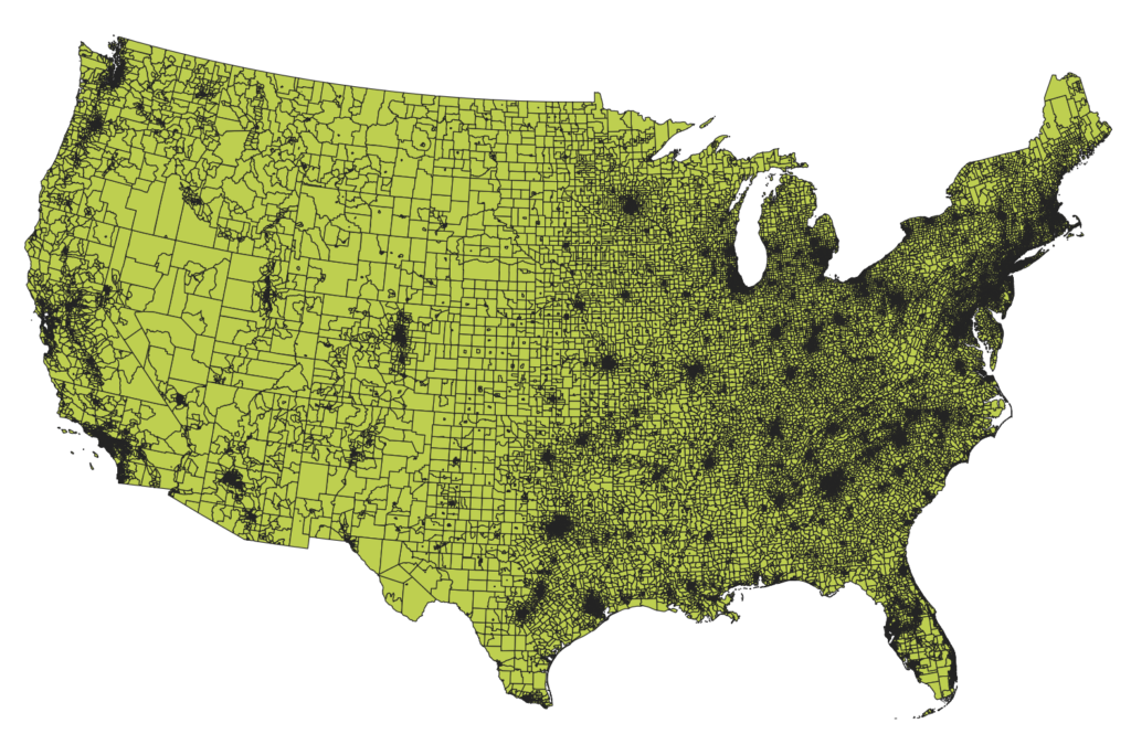
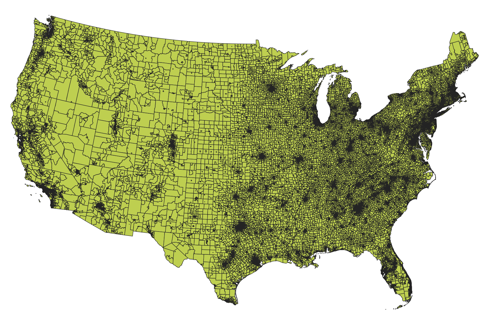
Getting national census data, with related geometry data to analyze, is more difficult than it should be. The various tools that have been released by Census Bureau are geared toward “advanced casual users” and not those doing spatial analysis. Older tools, like Data Ferrett, have been phased out while newer tools, like data.census.gov, are still incomplete. The Census Bureau has released an API which allows developers to create tools to access data, including geometries like tracts and block groups, directly from the Census.

We don’t encourage downloading national data right away as it can be overwhelming to try to understand trends or work out the kinks in our code. We often try to get a minimum working example (MWE) of a local area as a way to test out our code and test out our analysis. We’ll then expand our analysis to the entire nation. One major hurdle has been finding a way to quickly download the data we need, with their spatial geometry, so that we can move from MWE to final analysis.
We tend to do most of our data analysis and gathering in R. Whether we use R or python depends on the project, but we often prefer to do this type of spatial work in R, and specifically in RStudio. Luckily, Kyle Walker’s tidycensus and tigris packages provide us the tools we need to get this data. Further, we use furrr and purrr packages to take advantage of multi-threading capacity in modern processors so that we can download data about each state in different threads—at the same time. One huge advantage of doing it this way is that we keep things within the tidyverse and our data will be accessible using the sf package.
Here’s how we might go about doing that.
First, we’d load all the packages in and set the options we need. If you haven’t already done so, be sure to install the packages listed below. You’ll also need a Census API Key, but that is free and straightforward.
library(furrr) # multicore
library(purrr) # for reduce
library(tidycensus) # acs
library(tigris) # fips codes

options(tigris_class = "sf")
options(tigris_use_cache = TRUE)
census_api_key("YOUR CENSUS API KEY HERE")
Next we’ll need to get a list of all the states and DC in a string. We do that using tigris and fips_codes$states variable. State FIPS codes are ordered, but not they are not sequential. That means that the numerical code for Alabama (AL) is 01 and Alaska (AK) is 02 because they are the first two states when sorted alphabetically. The next state, listed alphabetically, is Arizona (AZ) but its FIPSs code is 04 even though it is the 3rd state. This leaves a convenient places for American Samoa (AS) whose current FIPS code is 52nd and is 60. Worth noting that the District of Columbia combined in the FIPS state level code and is 9th with a FIPS code of 11.
What does this mean for us? If we want to put together a list of states that includes DC, we can use the fips_codes$states variable to get the first 51 items (50 states and DC), because it’s sorted by FIPS code and not alphabetically (avoiding American Samoa). If we wanted to grab American Samoa, we simply wouldn’t subset our list. I’ve wrapped fips_codes in unique simply as a precaution and stored our list in fips.states.
fips.states <- unique(fips_codes$state)[1:51]
We also want to setup our multi-thread. We’re telling R to use all but one of available threads (which it refers to as a core). We then plan a “multisession” R call to use that number of cores which allows for simultaneous sessions from within R.
num_cores <- availableCores() - 1
print(paste("Thread count to use:", num_cores))
plan(multisession, workers = num_cores)
Let’s talk about the data that we’re going to gather. In this example, we going to ask for block group data from the Hispanic or Latino by Race table, as well as some information about housing units and household income. In this example, we using the ACS 2019 5-year data. We’ve also set geometry to be TRUE so that we create a national shapefile. We’re also ensuring that we download data in the wide format. Notice that the we have not specified the state, which is listed currently as x.
If you’re following along, the following won’t run, we’re just explaining what the get_acs function call looks like. However, it’s best to test out your function call with an example (get a MWE) before continuing to attempt to multi-thread it!
# DO NOT RUN
get_acs(geography = "block group",
            variables = c("pop" = "B03002_001", # Total
                          "pop_nhwhite" = "B03002_003", # NH White
                          "pop_nhblack" = "B03002_004", # NH Black
                          "popx_nhamind" = "B03002_005", # NH Am Ind
                          "popx_nhasian" = "B03002_006", # NH Asian
                          "popx_nhhwnpi" = "B03002_007", # NH Hawaiian/PI
                          "popx_nhother" = "B03002_008", # One Other
                          "popx_nhtwomr" = "B03002_009", # Two+
                          "pop_hispltx" = "B03002_012", # Hispanic/Latinx
                          "hu_total"  = "B25001_001", # Housing Units
                          "hu_totocc" = "B25003_001", # Housing Units - Occ
                          "hu_totown" = "B25003_002", # Housing Units - Owner Occ,
                          "hu_totrnt" = "B25003_003", # Housing Units - Renter Occ,
                          "hh_total" = "B19001_001", # Total number of households
                          "hh_medinc" = "B19013_001" # Median household income
            ),

            year = 2019,
            survey = "acs5",
            state = x,
            geometry = TRUE,
            output = "wide",
            keep_geo_vars = TRUE)
The magic comes when we wrap our get_acs call within first future_map and then reduce. future_map is what allows us to call get_acs simultaneously based on the number of threads are available on the computer. reduce is what allows us to combine all the results into a single spatial dataframe, in this case ntl_bg_sf.
Using future_map we tell R to run a bit of code for each item in the fips.states list we created earlier. Using function(x) lets us take each item, as the variable x, and run the wrapped get_acs function. This is why the in the get_acs function, state is set to x, that is we’re preparing to substitute x for each FIPS state abbreviation.
We do this by telling reduce to reduce the results by appending the rows of the results known as rbind. In this example, we’ve added comments in the R code to explain each of the steps.
ntl_bg_sf <- reduce(
  future_map(fips.states, function(x) {
    get_acs(geography = "block group",
            variables = c("pop" = "B03002_001", # Total
                          "pop_nhwhite" = "B03002_003", # NH White
                          "pop_nhblack" = "B03002_004", # NH Black
                          "popx_nhamind" = "B03002_005", # NH Am Ind
                          "popx_nhasian" = "B03002_006", # NH Asian
                          "popx_nhhwnpi" = "B03002_007", # NH Hawaiian/PI
                          "popx_nhother" = "B03002_008", # One Other
                          "popx_nhtwomr" = "B03002_009", # Two+
                          "pop_hispltx" = "B03002_012", # Hispanic/Latinx
                          "hu_total"  = "B25001_001", # Housing Units
                          "hu_totocc" = "B25003_001", # Housing Units - Occ
                          "hu_totown" = "B25003_002", # Housing Units - Owner Occ,
                          "hu_totrnt" = "B25003_003", # Housing Units - Renter Occ,
                          "hh_total" = "B19001_001", # Total number of households
                          "hh_medinc" = "B19013_001" # Median household income
            ),

            year = 2019,
            survey = "acs5",
            state = x,
            geometry = TRUE,
            output = "wide",
            keep_geo_vars = TRUE)
  }, .progress = TRUE), # show a progress bar associated with `future_map`
  rbind # rbind here is how we combine the different state results
  # it is part of the `reduce` function
)
How might you tweak this? In our example, we’ve set the geography to block group, but we could easily perform this call at the tract level if we needed. We could also subset the states or create a custom list of state abbreviations if, say, you only wanted particular regions. Obviously, we could have change the variables that we’re inspecting. Just be sure that data is available at the level of detail you are interested in. We highly recommend viewing examples on Kyle Walker’s site for tidycensus to get an idea of what is possible. Lastly, we like perusing available data and getting the variable names from Social Explorer’s Data Dictionary even though there are functions built write into tidycensus to do so.
Download the completed R script here. Don’t forget to include your own Census API Key in quotes.
We hope that you found this walk-through helpful and encourage you to check out our other guides. We’ll do our best to keep this updated and will post a new example once the 2020 census is released.
